|
'''
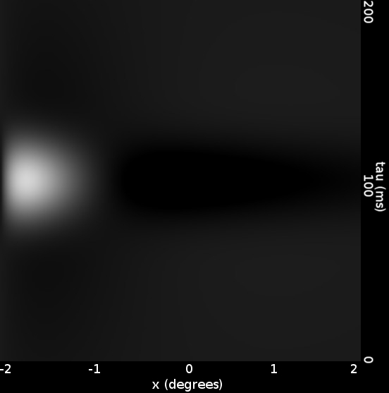
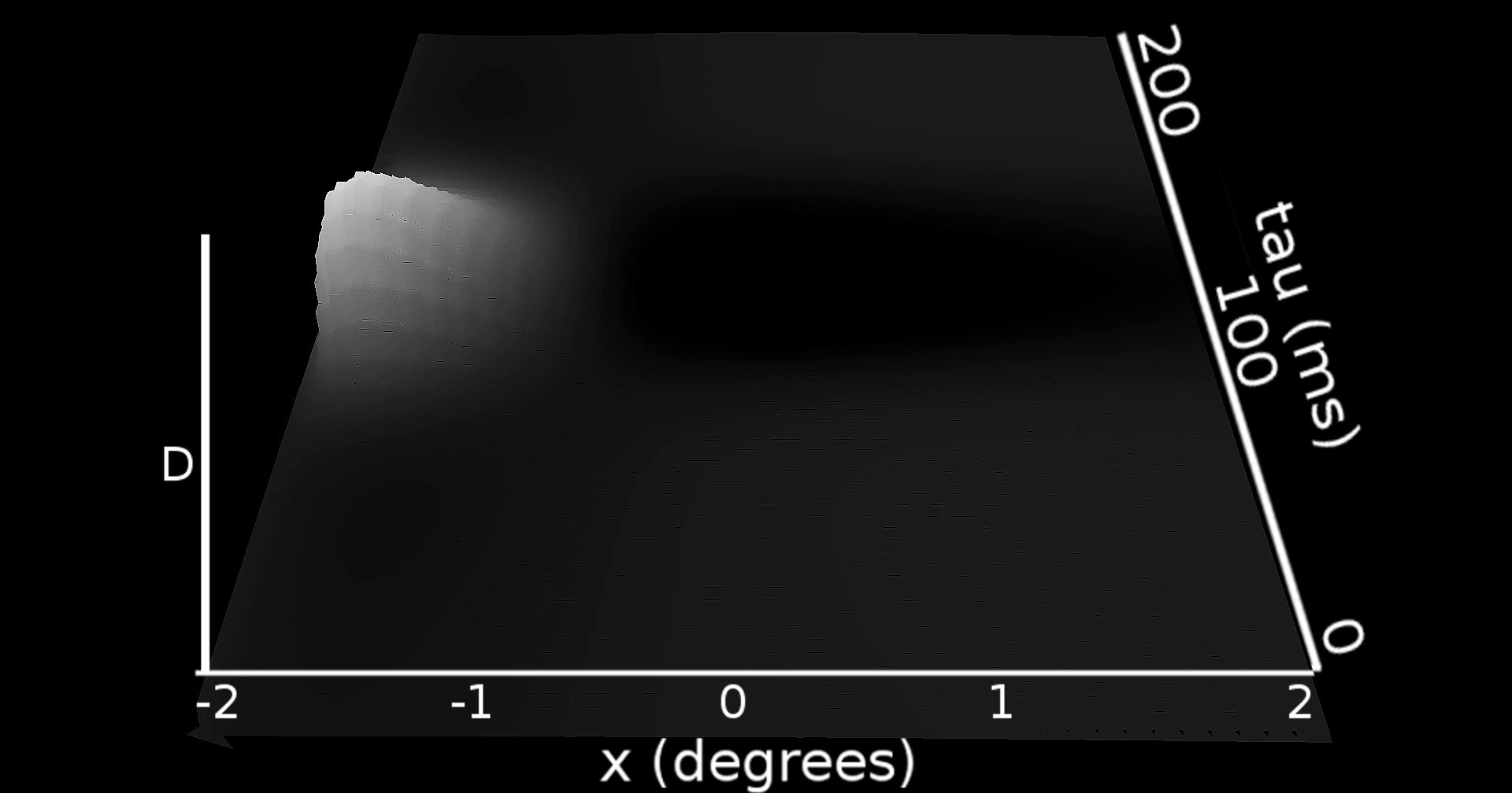
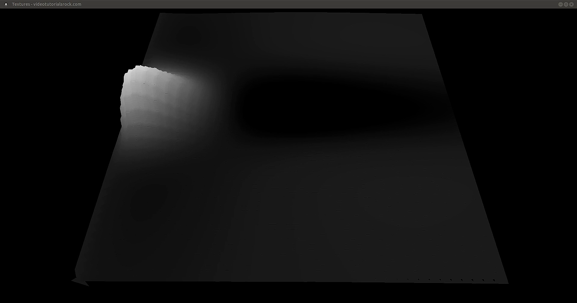
Temporal structure of a visual receptive feild.
This can simulate changes due to time of the fields
(Dayan and Abbott, pg 66)
'''
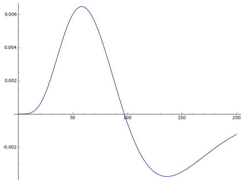
ms = .001
a = 1/15
tau = var('tau')
time = a*exp(-a*tau)*((((a*tau)^5)/factorial(5))-(((a*tau)^7)/factorial(7)))
plot(time, (tau,0,200))
|


.png "Click on 3-D image to make it live. Right-click on live image for a control menu.")
.png "Click on 3-D image to make it live. Right-click on live image for a control menu.")
.png "Click on 3-D image to make it live. Right-click on live image for a control menu.")
.png "Click on 3-D image to make it live. Right-click on live image for a control menu.")
.png "Click on 3-D image to make it live. Right-click on live image for a control menu.")
.png "Click on 3-D image to make it live. Right-click on live image for a control menu.")
.png "Click on 3-D image to make it live. Right-click on live image for a control menu.")
.png "Click on 3-D image to make it live. Right-click on live image for a control menu.")